InfraRed imaging Vedeo Bolometer

Synthetic diagnostics calculation of InfraRed imaging Vedeo Bolometer (IRVB).

Here is a demo program assuming for IRVB at ITER. The parameters for the IRVB are describled in IRVB_conf.yaml file as follows:

#################################################
##########    IRVB configuration    #############
#################################################
# setting parameters for:
#   1. IRVB camera
#   2. raysect
#   3. IMAS

# === 1. IRVB Camera Setting ==================================================
camera:
  C9:                       # camera variant
    Diag: IRVB_E12R         # diagnostics
    Name: IRVB_view_f=21cm  # user-specific name
    P: [-5.960767, -6.205868, 0.82] # centre position of slit (x, y, z)[m]
    F: 21.0e-2                      # focal length [m]
    D12: [7.0e-2, 9.0e-2]           # foil size (dx, dy) [m]
    N12: [28, 36]                   # pixel resolution
    nIn: [0.8365163037378079, 0.2241438680420134, -0.4999999999999998]  # direction verctor
    pixel_samples: 1000  # specific number of pixel samples


# === 2. Raysect ray-trace common setting =====================================
raysect:
  camera: C9  # camera variant
  reflection: False
  los_step: 1.0e-3  # line integration step [m]
  pixel_samples: 1000  # default number of pixel samples

  savedir: ../output  # destination
  
  
# === 3. IMAS setting =========================================================
ids:
  # ids fundamental parameters
  shot: 134000
  run:  15
  user: public
  database: iter

  # For core, edge_sources ids
  source: "radiation"
  particle: "electrons"

  # time (-1 means selecting the first one)
  time: -1

This yaml file must be put into the same folder as the python script.

Python script

module loading

import numpy as np
import matplotlib.pyplot as plt

from raysect.core import translate, Point3D, Vector3D, rotate_basis
from raysect.primitive import Cylinder
from raysect.optical import World
from raysect.optical.observer import PinholeCamera, PowerPipeline2D, MonoAdaptiveSampler2D
from raysect.optical.material import VolumeTransform, AbsorbingSurface

from cherab.tools.emitters import RadiationFunction
from cherab.iter.tools.visualization import plot_2D_data
from cherab.imas import EquilibriumIDS, CoreSourcesIDS, EdgeSourcesIDS
from cherab.iter.machine import import_iter_mesh

import yaml
import argparse

Define Initial condition

Load setting file (yaml)

with open("IRVB_conf.yaml", "r") as file:
    conf = yaml.safe_load(file)

# obtain arguments
parser = argparse.ArgumentParser()
parser.add_argument(
    "-c", "--camera", required=False, help="camera case must be choosed cases wiritten in conf.yaml"
)
parser.add_argument("--run", required=False, type=int, help="run number is IMAS ids run number")
args = parser.parse_args()

# IDS setting
SHOT = conf["ids"]["shot"]
if args.run:
    RUN = args.run
else:
    RUN = conf["ids"]["run"]
USER = conf["ids"]["user"]
DATABASE = conf["ids"]["database"]
SOURCE = conf["ids"]["source"]
PARTICLE = conf["ids"]["particle"]
TIME = conf["ids"]["time"]

# raysect setting
if args.camera:
    case = args.camera  # select camera case by arguments
else:
    case = conf["raysect"]["camera"]
print(f"Set camera: {conf['camera'][case]['Diag']} -case: {case}")
Reflection = conf["raysect"]["reflection"]
los_step = conf["raysect"]["los_step"]

Define radiation function

The radiation from plasma consists of loss of electron energy in edge and core region. Here we define the \((X, Y, Z)\) coordinates function.

print(f"importing shot:{SHOT}, run:{RUN}, source:'{SOURCE}', particle:'{PARTICLE}'")
equilibrium_ids = EquilibriumIDS(shot=SHOT, run=RUN, user=USER, database=DATABASE)
equi = equilibrium_ids.time(TIME)
core_sources = CoreSourcesIDS(shot=SHOT, run=RUN, user=USER, database=DATABASE)
edge_sources = EdgeSourcesIDS(shot=SHOT, run=RUN, user=USER, database=DATABASE)
# extract energy data
core_sources.energy(source=SOURCE, particle=PARTICLE, equilibrium=equi)
edge_sources.mesh().energy(source=SOURCE, particle=PARTICLE)
# create radiation distribution function
energy_2D = core_sources.map2d() + edge_sources.map2d()
energy_3D = core_sources.map3d() + edge_sources.map3d()

Create Primitives

# -------- set const. --------- #
# set plasma profile r,z range
RMIN, RMIN = edge_sources.r_range
ZMIN, ZMAX = edge_sources.z_range
CYLINDER_RADIUS = RMIN
CYLINDER_HEIGHT = ZMAX - ZMIN

# last wall r,z range (terminal absorbar)
WALL_RMIN = RMIN - 1.0
WALL_RMAX = RMIN + 1.0
WALL_ZMAX = ZMAX + 1.5
WALL_ZMIN = ZMIN - 1.0
# ----------------------------- #

# World
world = World()

# Cylinder as teminate wall
central_column = Cylinder(
    WALL_RMIN,
    WALL_ZMAX - WALL_ZMIN,
    material=AbsorbingSurface(),
    parent=world,
    transform=translate(0, 0, WALL_ZMIN),
)

# ITER PFC meshes
mesh = import_iter_mesh(world, reflection=Reflection)

# Plasma emitter
# We shift the cylinder containing the emission function relative to the world,
# so need to apply the opposite shift to the material to ensure the radiation
# function is evaluated in the correct coordinate system.
shift = translate(0, 0, ZMIN)
radiation_emitter = VolumeTransform(RadiationFunction(energy_3D, step=los_step), shift.inverse())

# Plasma
geom = Cylinder(
    CYLINDER_RADIUS, CYLINDER_HEIGHT, transform=shift, parent=world, material=radiation_emitter
)

Add IRVB camera as an Observer

Camera configuration (position, orientation, etc.) is loaded from yaml file. Pinhole is used as IRVB camera.

camera_pos = conf["camera"][f"{case}"]["P"]  # camera position
camera_ori = conf["camera"][f"{case}"]["nIn"]  # camera orientation
pixels = conf["camera"][f"{case}"]["N12"]  # pixel number
focal_length = conf["camera"][f"{case}"]["F"]  # focal length
pixel_size = conf["camera"][f"{case}"]["D12"]  # pixel size

# Field of view
fov = 2.0 * np.arctan(np.hypot(*pixel_size) / (2.0 * focal_length)) * 180 / np.pi  # [deg]

camera_pos = Point3D(*camera_pos)
camera_ori = Vector3D(*camera_ori)
camera_tran = translate(camera_pos.x, camera_pos.y, camera_pos.z)
camera_rot = rotate_basis(camera_ori, Vector3D(0, 0, 1))

# the number of pixel samples
try:
    min_samples = conf["camera"][f"{case}"]["pixel_samples"]
except NameError:
    min_samples = conf["raysect"]["pixel_samples"]

pipeline = PowerPipeline2D(name="radiation")
sampler = MonoAdaptiveSampler2D(
    pipeline, fraction=0.2, ratio=25.0, min_samples=min_samples, cutoff=0.1
)
# generate camera object as a pinhole camera
camera = PinholeCamera(
    (pixels[0], pixels[1]),
    fov=fov,
    pipelines=[pipeline],
    parent=world,
    transform=camera_tran * camera_rot,
    frame_sampler=sampler,
)

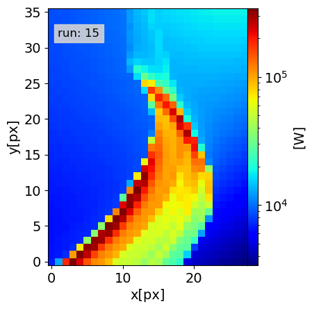
Excute ray tracing and Plot a simulated image

plt.ion()
camera.observe()
plt.ioff()

fig = plt.figure()
fig, grid = plot_2D_data(
    fig=fig,
    data=[np.rot90((pipeline.frame.mean), k=1)],
    ax_row=1,
    plot_mode="log",
    titles=[f"run: {RUN}"],
    clabel="[W]",
    title_params={"fontsize": 12, "y": 0.9},
)
plt.savefig("radiation_JINTRAC.png", bbox_inches="tight")
plt.show()