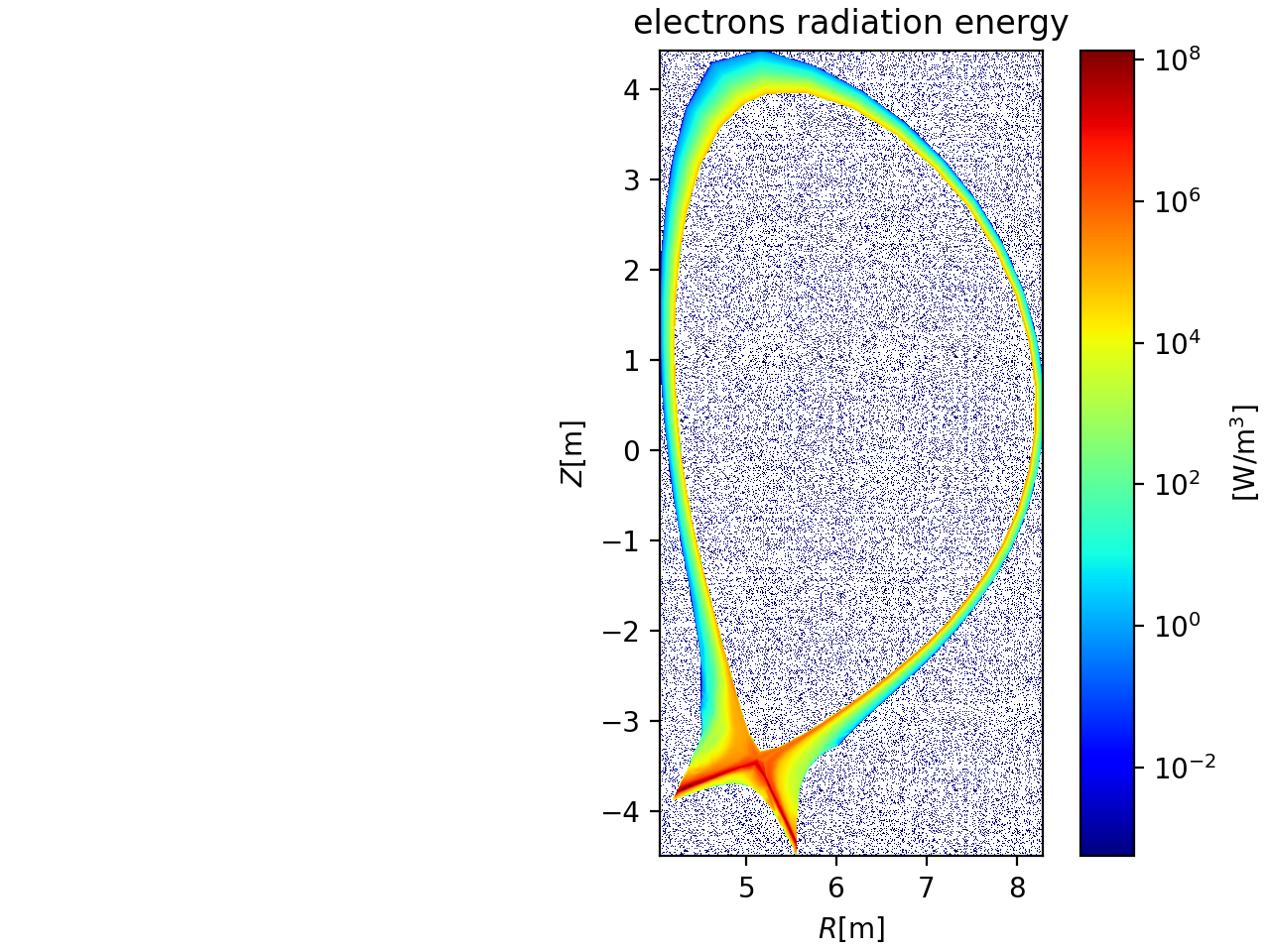
2D profiles stored in edge_sources ids

Out:

importing shot:134000, run:29, source:'radiation', particle:'electrons'
Sampling...
plotting 2D profiles...

import numpy as np
from matplotlib import pyplot as plt
from matplotlib.colors import LogNorm
from matplotlib.ticker import LogFormatterSciNotation, MultipleLocator

from cherab.core.math import sample2d
from cherab.imas import EdgeSourcesIDS


# IDS Setting
SHOT = 134000
RUN = 29
USER = "koyo"
DATABASE = "iter"

SOURCE = "radiation"
PARTICLE = "electrons"

print(f"importing shot:{SHOT}, run:{RUN}, source:'{SOURCE}', particle:'{PARTICLE}'")

# JINTRAC-SOLPS Case
edge_sources = EdgeSourcesIDS(shot=SHOT, run=RUN, user=USER, database=DATABASE)
energy = edge_sources.mesh().energy(source=SOURCE, particle=PARTICLE)
energy_2D = energy.map2d()

print("Sampling...")
rmin, rmax = edge_sources.r_range
zmin, zmax = edge_sources.z_range

resolution = 0.01  # sample every 1 cm
nr = int(round((rmax - rmin) / resolution))
nz = int(round((zmax - zmin) / resolution))

# sampling r,z, distibution
r, z, energy_samples = sample2d(energy_2D, (rmin, rmax, nr), (zmin, zmax, nz))

# plot
print("plotting 2D profiles...")
fig, ax = plt.subplots(constrained_layout=True)
im = ax.imshow(
    np.transpose(energy_samples),
    extent=[
        rmin - resolution * 0.5,
        rmax + resolution * 0.5,
        zmin - resolution * 0.5,
        zmax + resolution * 0.5
    ],
    cmap="jet",
    origin="lower",
    norm=LogNorm(),
)
# colorbar setting
cbar = plt.colorbar(im, ax=ax, label="[W/m$^3$]", format=LogFormatterSciNotation())
# axes setting
ax.xaxis.set_major_locator(MultipleLocator(1.0))  # set the axis major tickes to 1.0m width
ax.yaxis.set_major_locator(MultipleLocator(1.0))
ax.set_title(f"{PARTICLE} {SOURCE} energy")
ax.set_xlabel("$R$[m]")
ax.set_ylabel("$Z$[m]")

plt.show()