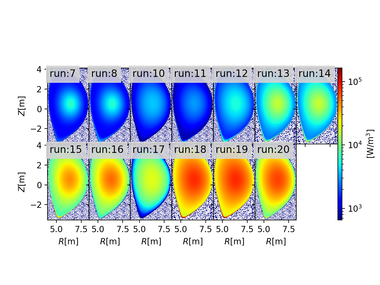
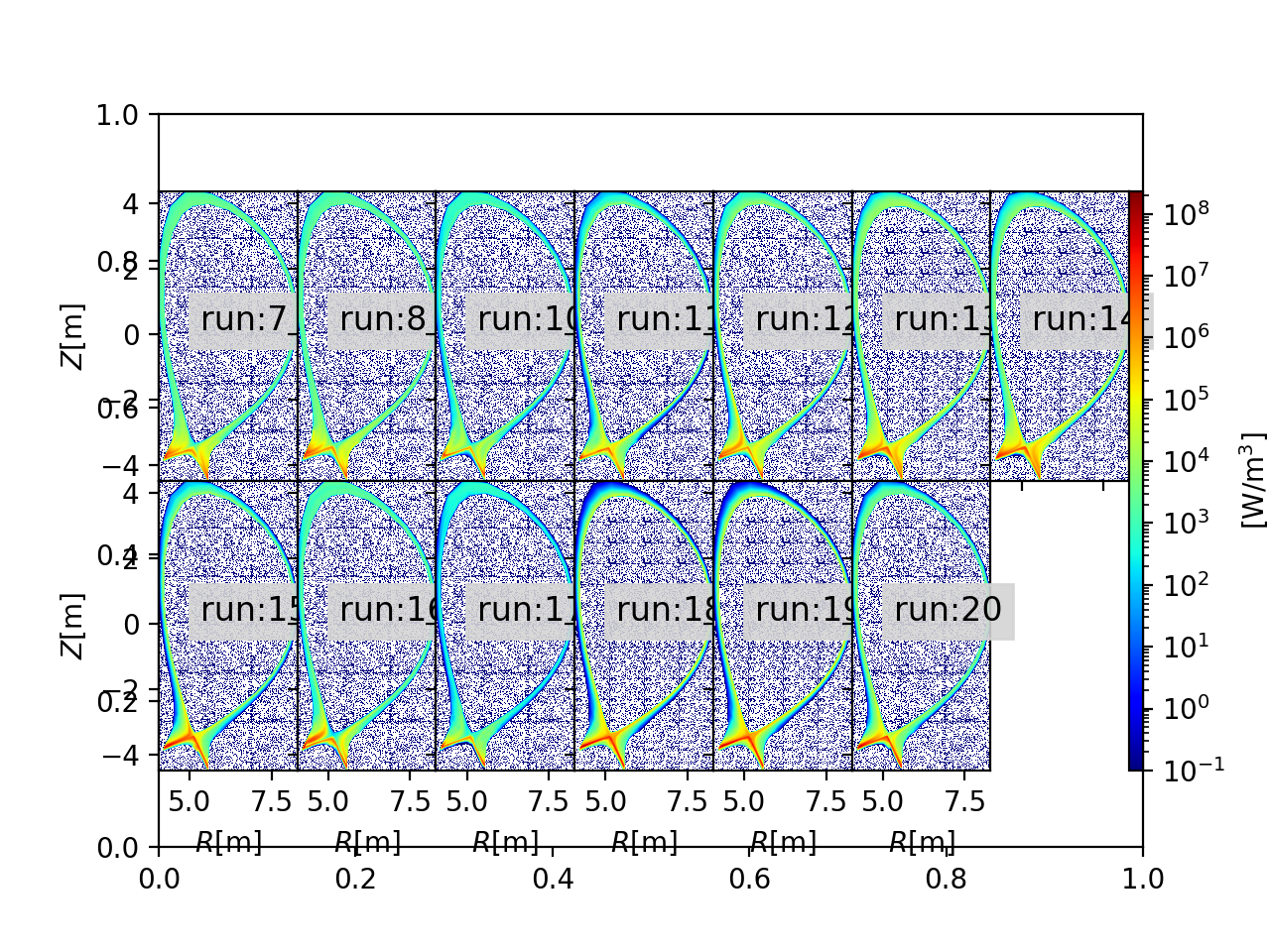
2D profiles generated by JINTRAC

• 
• 

Out:

importing shot:134000, run:7, source:'radiation', particle:'electrons'
importing shot:134000, run:8, source:'radiation', particle:'electrons'
importing shot:134000, run:10, source:'radiation', particle:'electrons'
importing shot:134000, run:11, source:'radiation', particle:'electrons'
importing shot:134000, run:12, source:'radiation', particle:'electrons'
importing shot:134000, run:13, source:'radiation', particle:'electrons'
importing shot:134000, run:14, source:'radiation', particle:'electrons'
importing shot:134000, run:15, source:'radiation', particle:'electrons'
importing shot:134000, run:16, source:'radiation', particle:'electrons'
importing shot:134000, run:17, source:'radiation', particle:'electrons'
importing shot:134000, run:18, source:'radiation', particle:'electrons'
importing shot:134000, run:19, source:'radiation', particle:'electrons'
importing shot:134000, run:20, source:'radiation', particle:'electrons'

from matplotlib import pyplot as plt

from cherab.core.math import sample2d
from cherab.imas import EquilibriumIDS, CoreSourcesIDS, EdgeSourcesIDS
from cherab.iter.tools.visualization import plot_2D_profile

# IDS Setting
SHOT = 134000
RUNs = [7, 8] + [i for i in range(10, 20 + 1)]

USER = "koyo"
DATABASE = "iter"

SOURCE = "radiation"
PARTICLE = "electrons"

data_core = []
data_edge = []

for RUN in RUNs:
    print(f"importing shot:{SHOT}, run:{RUN}, source:'{SOURCE}', particle:'{PARTICLE}'")

    equilibrium_ids = EquilibriumIDS(shot=SHOT, run=RUN, user=USER, database=DATABASE)
    imas_equilibrium = equilibrium_ids.time(-1)
    core_sources = CoreSourcesIDS(shot=SHOT, run=RUN, user=USER, database=DATABASE)
    edge_sources = EdgeSourcesIDS(shot=SHOT, run=RUN, user=USER, database=DATABASE)
    core_sources.energy(source=SOURCE, particle=PARTICLE, equilibrium=imas_equilibrium)
    edge_sources.mesh().energy(source=SOURCE, particle=PARTICLE)
    # generate 2D function
    core_2D = core_sources.map2d()
    edge_2D = edge_sources.map2d()

    # sampling limit
    core_lim = {"xlim": imas_equilibrium.r_range, "ylim": imas_equilibrium.z_range}
    edge_lim = {"xlim": edge_sources.r_range, "ylim": edge_sources.z_range}

    # sample every 1 cm
    resolution = 0.01
    nr_core = int(round((core_lim["xlim"][1] - core_lim["xlim"][0]) / resolution))
    nz_core = int(round((core_lim["ylim"][1] - core_lim["ylim"][0]) / resolution))
    nr_edge = int(round((edge_lim["xlim"][1] - edge_lim["xlim"][0]) / resolution))
    nz_edge = int(round((edge_lim["ylim"][1] - edge_lim["ylim"][0]) / resolution))

    # sampling r,z, distibution
    r_core, z_core, core = sample2d(
        core_2D, (*core_lim["xlim"], nr_core), (*core_lim["ylim"], nz_core)
    )
    r_edge, z_edge, edge = sample2d(
        edge_2D, (*edge_lim["xlim"], nr_edge), (*edge_lim["ylim"], nz_edge)
    )
    core[core < 0] = 0
    edge[edge < 0] = 0
    data_core.append(core)
    data_edge.append(edge)

# plot
plot_mode = "log"
ax_row = 2
fig1 = plt.figure()
fig2 = plt.figure()
plot_2D_profile(
    fig=fig1,
    data=data_core,
    xdata=r_core,
    ydata=z_core,
    ax_row=ax_row,
    title=[f"run:{run}" for run in RUNs],
    titlekw={"fontsize": 12, "y": 0.92},
    plot_mode=plot_mode,
)
plot_2D_profile(
    fig=fig2,
    data=data_edge,
    vmin=1.0e-1,
    xdata=r_edge,
    ydata=z_edge,
    ax_row=ax_row,
    title=[f"run:{run}" for run in RUNs],
    titlekw={"fontsize": 12, "x": 0.30, "y": 0.55},
    plot_mode=plot_mode,
)
plt.show()