Polar BRDF Plots

This example demonstrates how to sample the BRDFs of materials with the evaluate_shading() method.

import matplotlib.pyplot as plt
import numpy as np

from raysect.core import AffineMatrix3D, Point3D, Vector3D
from raysect.optical import Ray, World
from raysect.optical.library.metal import RoughAluminium
from raysect.optical.material import UnitySurfaceEmitter
from raysect.primitive import Sphere

# Create scene graph
world = World()
ray = Ray(min_wavelength=500, max_wavelength=500.1, bins=1)
sphere = Sphere(100, parent=world, material=UnitySurfaceEmitter())

# Define Consts.
origin = Point3D(0, 0, 0)
material = RoughAluminium(0.25)
thetas = np.linspace(-90, 90, 100)

plt.ion()
for light_angle in [0, -25, -45, -70]:
    light_position = Point3D(
        np.sin(np.deg2rad(light_angle)), 0, np.cos(np.deg2rad(light_angle))
    )
    light_direction = origin.vector_to(light_position).normalise()

    brdfs = []
    for theta_step in thetas:
        detector_position = Point3D(
            np.sin(np.deg2rad(theta_step)), 0, np.cos(np.deg2rad(theta_step))
        )
        detector_direction = origin.vector_to(detector_position).normalise()

        # Calculate spectrum
        spectrum = material.evaluate_shading(
            world,
            ray,
            light_direction,
            detector_direction,
            origin,
            origin,
            False,
            AffineMatrix3D(),
            AffineMatrix3D(),
            None,
        )
        brdfs.append(spectrum.samples[0])

    plt.plot(thetas, brdfs, label="{} degrees".format(light_angle))

plt.xlabel("Observation Angle (degrees)")
plt.ylabel("BRDF() (probability density)")
plt.legend()
plt.title("The Aluminium BRDF VS observation angle")


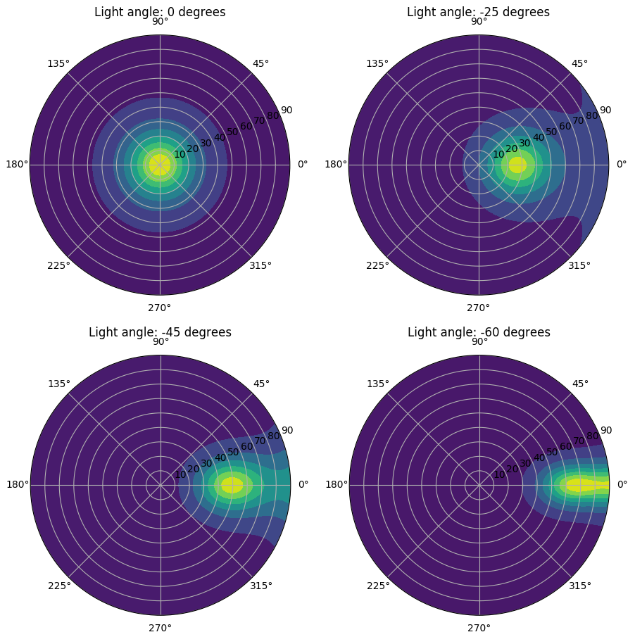
def plot_brdf(light_angle):
    light_position = Point3D(
        np.sin(np.deg2rad(light_angle)), 0, np.cos(np.deg2rad(light_angle))
    )
    light_direction = origin.vector_to(light_position).normalise()

    phis = np.linspace(0, 360, 200)
    num_phis = len(phis)
    thetas = np.linspace(0, 90, 100)
    num_thetas = len(thetas)

    values = np.zeros((num_thetas, num_phis))
    for i, j in np.ndindex(num_thetas, num_phis):
        theta = np.deg2rad(thetas[i])
        phi = np.deg2rad(phis[j])
        outgoing = Vector3D(
            np.cos(phi) * np.sin(theta), np.sin(phi) * np.sin(theta), np.cos(theta)
        )

        # Calculate spectrum
        spectrum = material.evaluate_shading(
            world,
            ray,
            light_direction,
            outgoing,
            origin,
            origin,
            False,
            AffineMatrix3D(),
            AffineMatrix3D(),
            None,
        )
        values[i, j] = spectrum.samples[0]

    fig, ax = plt.subplots(subplot_kw=dict(projection="polar"))
    cs = ax.contourf(np.deg2rad(phis), thetas, values, extend="both")
    cs.cmap.set_under("k")
    plt.title("Light angle: {} degrees".format(light_angle))


plot_brdf(0)
plot_brdf(-25)
plot_brdf(-45)
plot_brdf(-60)
plt.ioff()
plt.show()