Ray Logging Trajectories
This demonstration visualises full ray trajectories through a simple optical system. The scene contains a symmetric bi-convex lens made of Schott N-BK7 glass (used in transmission-only mode) and a large absorbing target plane positioned behind the lens to terminate rays.
For each starting position on a small grid in front of the lens, a
LoggingRay is traced through the scene. At every interaction with a
surface, the ray records the intersection hit point. After tracing, the
logged points are plotted in 3D with matplotlib as both a polyline
(black) and discrete markers (red), revealing how rays refract and where
they intersect geometry.
See also Ray Intersection Points for a related example that records only the first intersection point for each ray.
# External imports
import matplotlib.pyplot as plt
import numpy as np

# Raysect imports
from raysect.optical import Point3D, Vector3D, World, translate
from raysect.optical.library import schott
from raysect.optical.loggingray import LoggingRay
from raysect.optical.material.absorber import AbsorbingSurface
from raysect.primitive import Box
from raysect.primitive.lens.spherical import BiConvex

world = World()

# Create a glass BiConvex lens we want to study
lens_glass = schott("N-BK7")
lens_glass.transmission_only = True
lens = BiConvex(0.0254, 0.0052, 0.0506, 0.0506, parent=world, material=lens_glass)

# Create a target plane behind the lens.
target = Box(lower=Point3D(-50, -50, -0), upper=Point3D(50, 50, 0), material=AbsorbingSurface(),
             transform=translate(0, 0, 0.1), parent=world)


# for each sample direction trace a logging ray and plot the ray trajectory
plt.ion()
ax = plt.axes(projection='3d')

for u in np.linspace(-0.006, 0.006, 5):
    for v in np.linspace(-0.012, 0.012, 11):

        start = Point3D(v, u, -0.05)
        log_ray = LoggingRay(start, Vector3D(0, 0, 1))
        log_ray.trace(world)

        p = [(start.x, start.y, start.z)]
        for intersection in log_ray.log:
            point = intersection.hit_point
            p.append((point.x, point.y, point.z))
        p = np.array(p)

        ax.plot(p[:, 0], p[:, 1], p[:, 2], 'k-')
        ax.plot(p[:, 0], p[:, 1], p[:, 2], 'r.')

ax.set(
    xlabel="$X$",
    ylabel="$Y$",
    zlabel="$Z$",
)
plt.ioff()
plt.show()
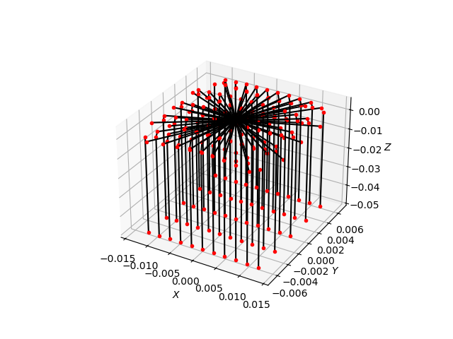
Ray trajectories are logged and visualised in 3D space. Rays start on a grid in front of the lens, refract through the lens, and are absorbed by the target plane. Red dots indicate ray-surface intersection points and black lines show the full ray paths.